Análisis de Área Bajo la Curva de Progreso de la Enfermedad (AUDPC)
¿Qué es el AUDPC?
El Área Bajo la Curva de Progreso de la Enfermedad (AUDPC, por sus siglas en inglés) es una medida utilizada en fitopatología para cuantificar el progreso de enfermedades en plantas a lo largo del tiempo. Esta métrica es ampliamente utilizada para comparar la severidad y el impacto de enfermedades entre diferentes tratamientos, variedades de plantas, o condiciones ambientales.
¿Cómo se Calcula el AUDPC?
El AUDPC se calcula a partir de observaciones repetidas de la severidad de la enfermedad en diferentes momentos del tiempo. La fórmula general para el cálculo del AUDPC es:
Donde: - y_i es la severidad de la enfermedad en el momento t_i. - t_i es el tiempo de la i-ésima observación. - n es el número total de observaciones.
Importancia del AUDPC
Comparación de Tratamientos:
Permite comparar la eficacia de diferentes tratamientos en el control de enfermedades.
Ayuda a identificar qué tratamiento ofrece la mejor protección contra una enfermedad específica.
Evaluación de Variedades de Plantas:
Utilizado para evaluar la resistencia de diferentes variedades de plantas a una enfermedad.
Ayuda a los fitomejoradores a seleccionar variedades más resistentes para programas de mejoramiento.
Monitoreo del Progreso de la Enfermedad:
Proporciona una visión general del progreso de la enfermedad a lo largo del tiempo.
Permite a los investigadores y agricultores tomar decisiones informadas sobre el manejo de la enfermedad.
Investigación y Desarrollo:
Fundamental en estudios de epidemiología vegetal y en la investigación sobre la dinámica de las enfermedades.
Ayuda a entender cómo diferentes factores (ambientales, genéticos, etc.) afectan el desarrollo de la enfermedad.
Ejemplo Práctico en R
Aquí hay un ejemplo práctico de cómo calcular el AUDPC utilizando R, usando un conjunto de datos ficticio sobre la severidad de una enfermedad en diferentes días.
La AUDPC es una medida utilizada para cuantificar el progreso de enfermedades en plantas a lo largo del tiempo.
    Welch Two Sample t-test

data:  curve3$Drip and curve3$Furrow
t = -1.3773, df = 3.079, p-value = 0.26
alternative hypothesis: true difference in means is not equal to 0
95 percent confidence interval:
 -1.3421436  0.5231436
sample estimates:
mean of x mean of y
 13.38983  13.79933
Interpretación de Resultados
Visualización Gráfica:
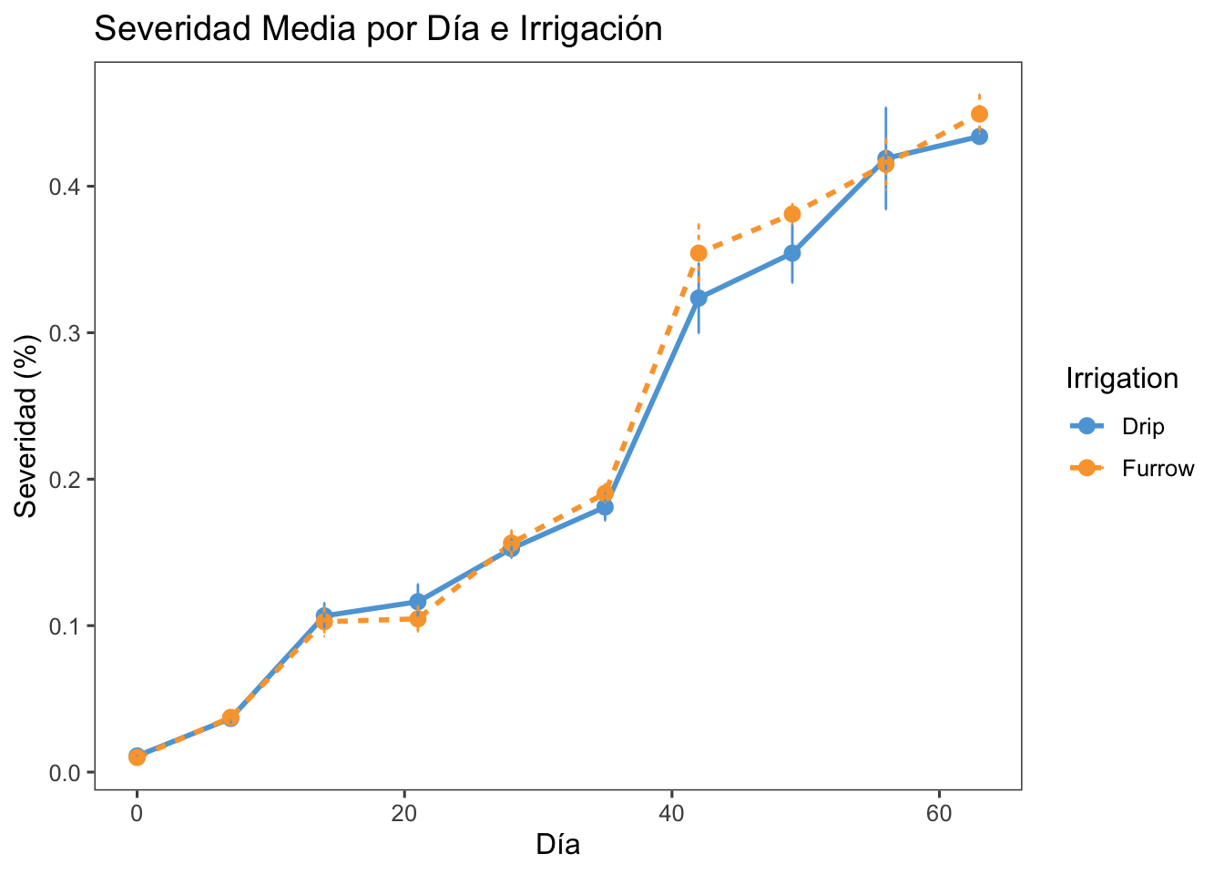
El gráfico muestra la severidad media de la enfermedad a lo largo del tiempo para diferentes tratamientos de irrigación.
Las barras de error indican la variabilidad de las observaciones.
Prueba t:
La prueba t compara las medias de AUDPC entre dos tratamientos de irrigación (por ejemplo, riego por goteo y riego por surco).
Un resultado significativo indicaría una diferencia estadísticamente significativa en el progreso de la enfermedad entre los dos tratamientos.
Ejercicio Práctico: irrigación
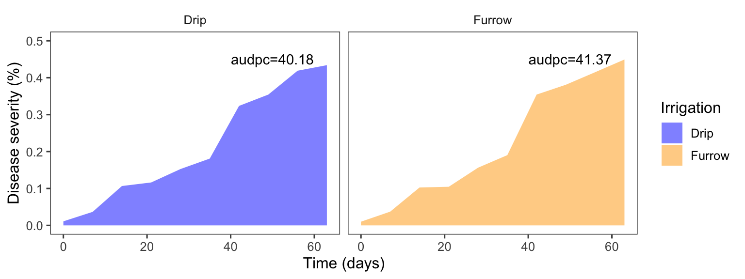
Cálculo del AUDPC:
La función AUDPC calcula el área bajo la curva de progreso de la enfermedad para cada combinación de tratamiento y repetición.
Valores más altos de AUDPC indican un mayor progreso de la enfermedad, mientras que valores más bajos indican un menor progreso.
Esta guía te ha mostrado cómo visualizar los resultados y cómo llevar a cabo análisis adicionales como AUDPC y ANOVA. Utilizando estas herramientas, puedes analizar y entender mejor tus datos categóricos y sus relaciones.
Si tienes alguna pregunta adicional o necesitas más ayuda con tu análisis, no dudes en preguntar.
Source Code
## Análisis de Área Bajo la Curva de Progreso de la Enfermedad (AUDPC)### ¿Qué es el AUDPC?El Área Bajo la Curva de Progreso de la Enfermedad (AUDPC, por sus siglas en inglés) es una medida utilizada en fitopatología para cuantificar el progreso de enfermedades en plantas a lo largo del tiempo. Esta métrica es ampliamente utilizada para comparar la severidad y el impacto de enfermedades entre diferentes tratamientos, variedades de plantas, o condiciones ambientales.### ¿Cómo se Calcula el AUDPC?El AUDPC se calcula a partir de observaciones repetidas de la severidad de la enfermedad en diferentes momentos del tiempo. La fórmula general para el cálculo del AUDPC es:`AUDPC = sum_{i=1}^{n-1} ({y_{i+1} + y_i}{2}) (t_{i+1} - t_i)`Donde: - `y_i` es la severidad de la enfermedad en el momento `t_i`. - `t_i` es el tiempo de la `i`-ésima observación. - `n` es el número total de observaciones.### Importancia del AUDPC1. **Comparación de Tratamientos**: - Permite comparar la eficacia de diferentes tratamientos en el control de enfermedades. - Ayuda a identificar qué tratamiento ofrece la mejor protección contra una enfermedad específica.2. **Evaluación de Variedades de Plantas**: - Utilizado para evaluar la resistencia de diferentes variedades de plantas a una enfermedad. - Ayuda a los fitomejoradores a seleccionar variedades más resistentes para programas de mejoramiento.3. **Monitoreo del Progreso de la Enfermedad**: - Proporciona una visión general del progreso de la enfermedad a lo largo del tiempo. - Permite a los investigadores y agricultores tomar decisiones informadas sobre el manejo de la enfermedad.4. **Investigación y Desarrollo**: - Fundamental en estudios de epidemiología vegetal y en la investigación sobre la dinámica de las enfermedades. - Ayuda a entender cómo diferentes factores (ambientales, genéticos, etc.) afectan el desarrollo de la enfermedad.### Ejemplo Práctico en RAquí hay un ejemplo práctico de cómo calcular el AUDPC utilizando R, usando un conjunto de datos ficticio sobre la severidad de una enfermedad en diferentes días.La AUDPC es una medida utilizada para cuantificar el progreso de enfermedades en plantas a lo largo del tiempo.### Cargar Paquetes```{r}library(datapasta)library(janitor)library(gsheet)library(googlesheets4)library(tidyverse)library(gsheet)library(cowplot)library(patchwork)library(ggthemes)library(epifitter)library(ggplot2)library(nlme)library(lme4)library(DHARMa)library(performance)library(report)library(emmeans)library(multcompView)library(multcomp)library(corrplot)library(see)library(lubridate)library(agridat)library(cowplot)library(agricolae)library(sf)library(broom)library(lattice)library(car)library(scales)library(readxl)library(dplyr)library(knitr)library(kableExtra)library(easyanova)library(tidyr)library(PerformanceAnalytics)library(magrittr)library(car)library(ggpubr)library(rstatix)library(reshape)library(kableExtra)library(formattable)library(sjPlot)library(sjlabelled)library(sjmisc)library(ggh4x)library(gridExtra)library(stringr)library(epiR)library(ggridges)library(DT)library(agricolae)library(ec50estimator)library(readxl)library(tidyverse)library(report)library(rstatix)```### Cargar Datos y Agrupar```{r}curve <-read_excel("dados-diversos.xlsx", sheet ="curve")curve|> DT::datatable(extensions ='Buttons', options =list(dom ='Bfrtip', buttons =c('excel', "csv")))```Vamos a cargar un archivo Excel que contiene los datos de severidad de la enfermedad y luego los agrupamos por tratamientos y días.```{r}curve2 <- curve |>group_by(Irrigation, day) |>summarize(mean_severity =mean(severity),sd_severity =sd(severity))curve2|> DT::datatable(extensions ='Buttons', options =list(dom ='Bfrtip', buttons =c('excel', "csv"))) |>formatRound(c('mean_severity','sd_severity'), 2)```### Visualizar AUDPC```{r}curve2 |>ggplot (aes(day, mean_severity, linetype = Irrigation, shape = Irrigation, group = Irrigation, color=Irrigation))+geom_line(linewidth =1)+geom_point(size =3, shape =16)+geom_errorbar(aes(ymin = mean_severity - sd_severity, ymax = mean_severity + sd_severity), width =0.1) +labs(title ="Severidad Media por Día e Irrigación",x ="Día",y ="Severidad (%)")+theme_few()+scale_color_few()```### Calcular AUDPC y Comparar```{r}curve3 <- curve |>group_by(Irrigation, rep) |>summarise(audpc =AUDPC(day, severity, y_proportion =FALSE)) |>pivot_wider(names_from = Irrigation, values_from = audpc)curve3|> DT::datatable(extensions ='Buttons', options =list(dom ='Bfrtip', buttons =c('excel', "csv")))|>formatRound(c('Drip','Furrow'), 2)``````{r}t.test(curve3$Drip, curve3$Furrow)```### Interpretación de Resultados- **Visualización Gráfica**: - El gráfico muestra la severidad media de la enfermedad a lo largo del tiempo para diferentes tratamientos de irrigación. - Las barras de error indican la variabilidad de las observaciones.- **Prueba t**: - La prueba t compara las medias de AUDPC entre dos tratamientos de irrigación (por ejemplo, riego por goteo y riego por surco). - Un resultado significativo indicaría una diferencia estadísticamente significativa en el progreso de la enfermedad entre los dos tratamientos.### Ejercicio Práctico: irrigación- **Cálculo del AUDPC**: - La función `AUDPC` calcula el área bajo la curva de progreso de la enfermedad para cada combinación de tratamiento y repetición. - Valores más altos de AUDPC indican un mayor progreso de la enfermedad, mientras que valores más bajos indican un menor progreso.```{r}library(epifitter)dat1 <- curve |>group_by(Irrigation,rep) |>summarize( audpc=AUDPC(day,severity))dat1t<-63dat1_audpc <- dat1 |>mutate(audpc2 = audpc / t)dat1_audpc dat1_audpc |> DT::datatable(extensions ='Buttons', options =list(dom ='Bfrtip', buttons =c('excel', "csv")))|>formatRound(c("audpc","audpc2"),2)``````{r}dat1_audpc_f<- dat1_audpc |>group_by(Irrigation) |>summarize(audpc =sum(audpc),TPD=mean(audpc2))dat1_audpc_f |> DT::datatable(extensions ='Buttons', options =list(dom ='Bfrtip', buttons =c('excel', "csv")))|>formatRound(c("audpc","TPD"),2)``````{r,fig.width=8, fig.height=3,fig.fullwidth=TRUE}f_labels <- data.frame(Irrigation = c("Drip", "Furrow"), label = c("audpc=40.18", "audpc=41.37"))curve |> group_by(Irrigation,day) |> summarise(severity=mean(severity)) |> ggplot (aes(day, severity, fill= Irrigation, group= Irrigation)) + geom_area(stat = "identity",position=position_identity(),alpha= 0.5)+ scale_fill_manual(values=c("Drip"="blue","Furrow"="orange"))+ theme_few()+ facet_wrap(~Irrigation)+ labs(y = "Disease severity (%)", x = "Time (days)")+ ylim(0,.5)+ geom_text(x = 50, y = .45, aes(label = label), data = f_labels)``````{r}anova_curve<-lm(audpc~ Irrigation +factor(rep), data = dat1_audpc )anova(anova_curve)``````{r}cv.model(anova_curve)```### Ejercicio Práctico: Lesion Size### Cargar y Manipular Datos```{r}lesion_size <-read_excel("tan-spot-wheat.xlsx", sheet ="lesion_size")lesion_size|> DT::datatable(extensions ='Buttons', options =list(dom ='Bfrtip', buttons =c('excel', "csv")))|>formatRound("lesion_size", 2)``````{r}lesion2 <- lesion_size |>mutate(lesion_size =as.numeric(lesion_size)) |>group_by(cult, silicio, hai) |>summarise(mean_lesion =mean(lesion_size), sd_lesion =sd(lesion_size))lesion2|> DT::datatable(extensions ='Buttons', options =list(dom ='Bfrtip', buttons =c('excel', "csv")))|>formatRound(c('mean_lesion','sd_lesion'), 2)```### Visualizar Datos```{r}lesion2 |>ggplot(aes(hai, mean_lesion,linetype = silicio, shape = silicio, group =silicio, color = silicio)) +geom_line(linewidth =1)+geom_point(size =3, shape =16)+geom_errorbar(aes(ymin = mean_lesion - sd_lesion, ymax = mean_lesion + sd_lesion), width =0.1) +facet_wrap(~cult) +labs(y ="Tamaño de Lesión (mm)",x ="Horas Después de Inoculación (hai)")+theme_few()+scale_color_few()```### Calcular AUDPC y Visualizar```{r}lesion3 <- lesion_size |>mutate(lesion_size =as.numeric(lesion_size)) |>group_by(exp, cult, silicio, rep) |>summarise(audpc =AUDPC(lesion_size, hai))lesion3|> DT::datatable(extensions ='Buttons', options =list(dom ='Bfrtip', buttons =c('excel', "csv")))|>formatRound("audpc", 2)``````{r}lesion3 |>ggplot(aes(cult, audpc, fill = silicio)) +geom_boxplot() +facet_wrap(~ exp)+theme_few()+scale_fill_few()```### Análisis ANOVA#### Realizar ANOVA```{r}aov1 <-aov(audpc ~ exp * cult * silicio, data = lesion3)summary(aov1)```#### Chequear Premisas```{r}check_normality(aov1)``````{r}check_heteroscedasticity(aov1)```#### Transformar Datos (si es necesario) y Verificar Medias```{r}aov1 <-aov(sqrt(audpc) ~ cult * silicio, data = lesion3)summary(aov1)``````{r}check_normality(aov1)``````{r}check_heteroscedasticity(aov1)``````{r}m1 <-cld(emmeans(aov1, ~ cult | silicio, type ="response"),alpha =0.05, Letters = LETTERS,reverse=F)m1 |> DT::datatable(extensions ='Buttons', options =list(dom ='Bfrtip', buttons =c('excel', "csv"))) |>formatRound(c('response','SE','lower.CL','upper.CL'), 2)```### Aprendizaje del DíaEsta guía te ha mostrado cómo visualizar los resultados y cómo llevar a cabo análisis adicionales como AUDPC y ANOVA. Utilizando estas herramientas, puedes analizar y entender mejor tus datos categóricos y sus relaciones.Si tienes alguna pregunta adicional o necesitas más ayuda con tu análisis, no dudes en preguntar.